BOW: Bayesian Optimization over Windows for Motion Planning in Complex Environments

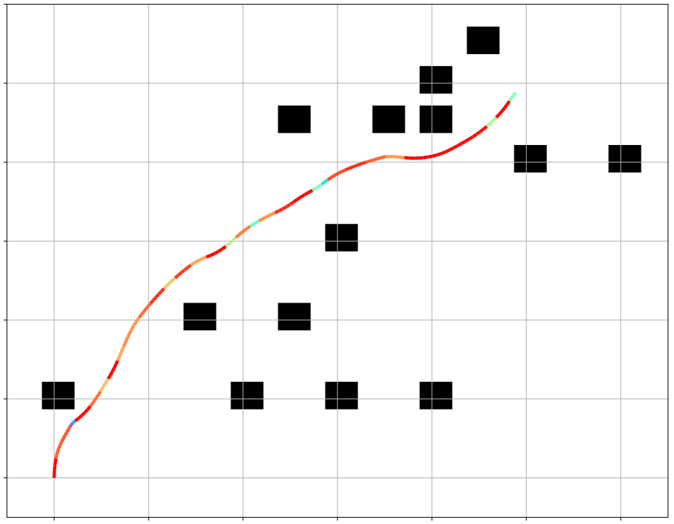
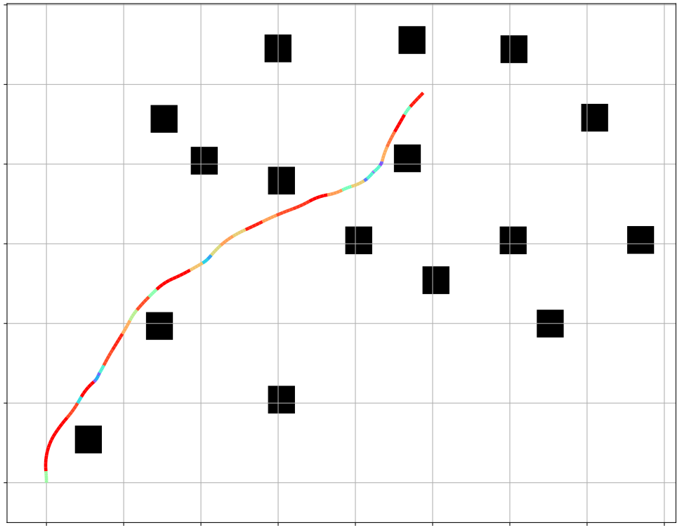
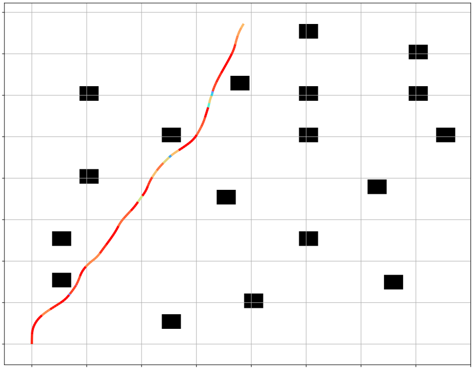
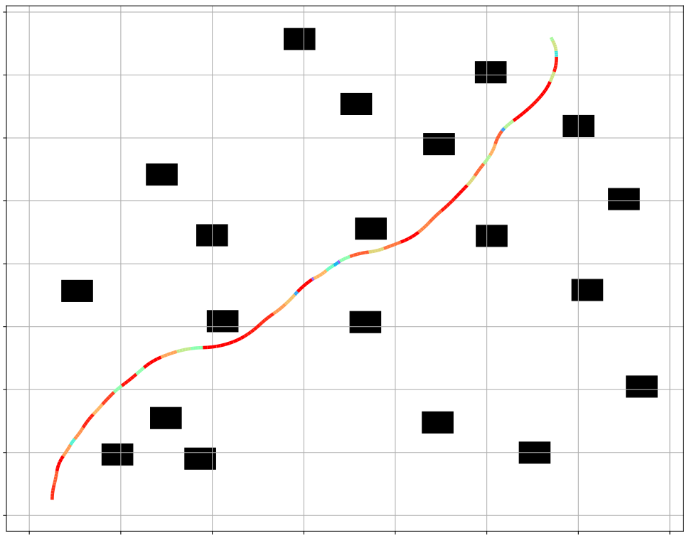
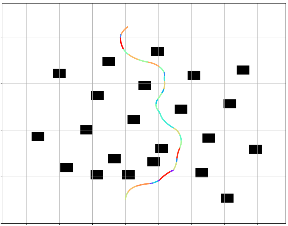
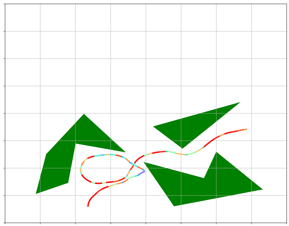
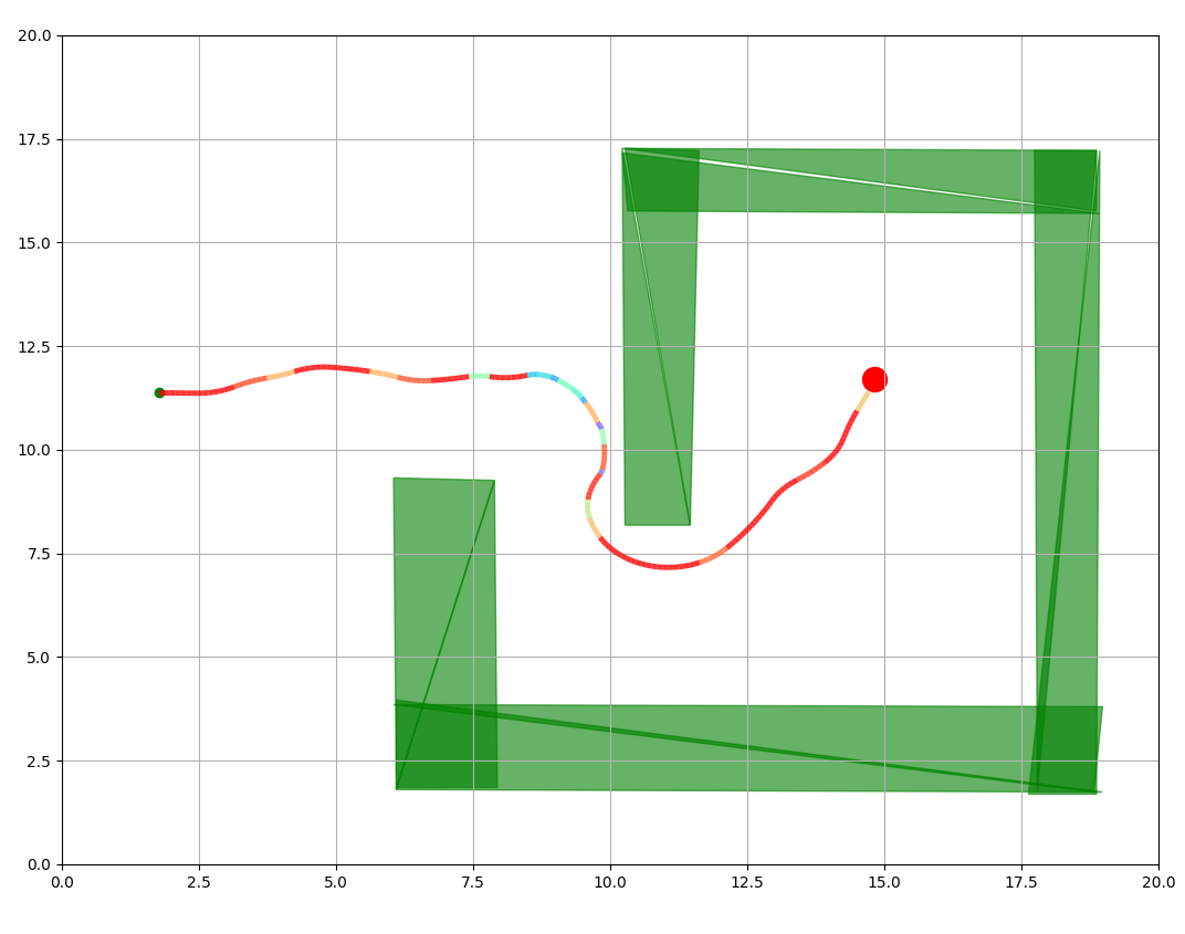
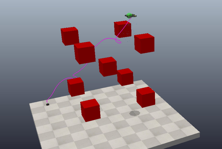
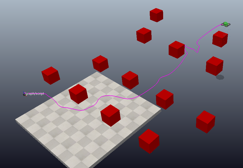
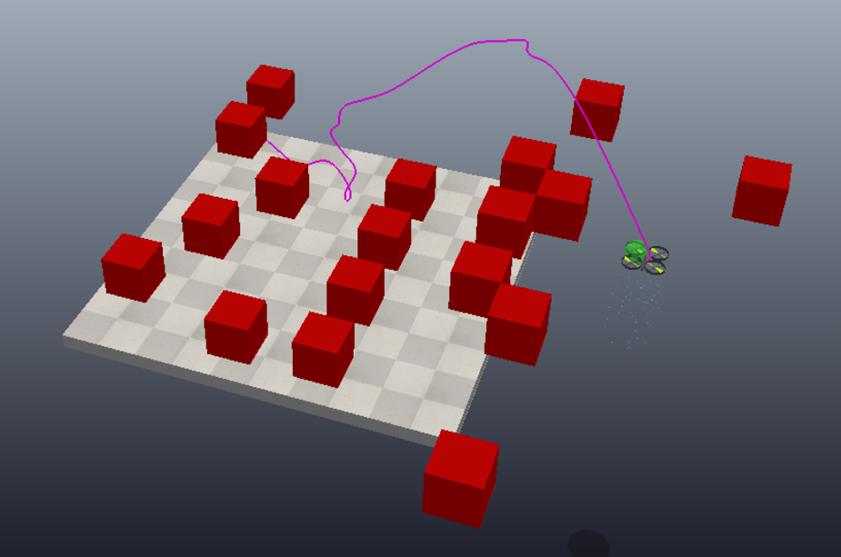
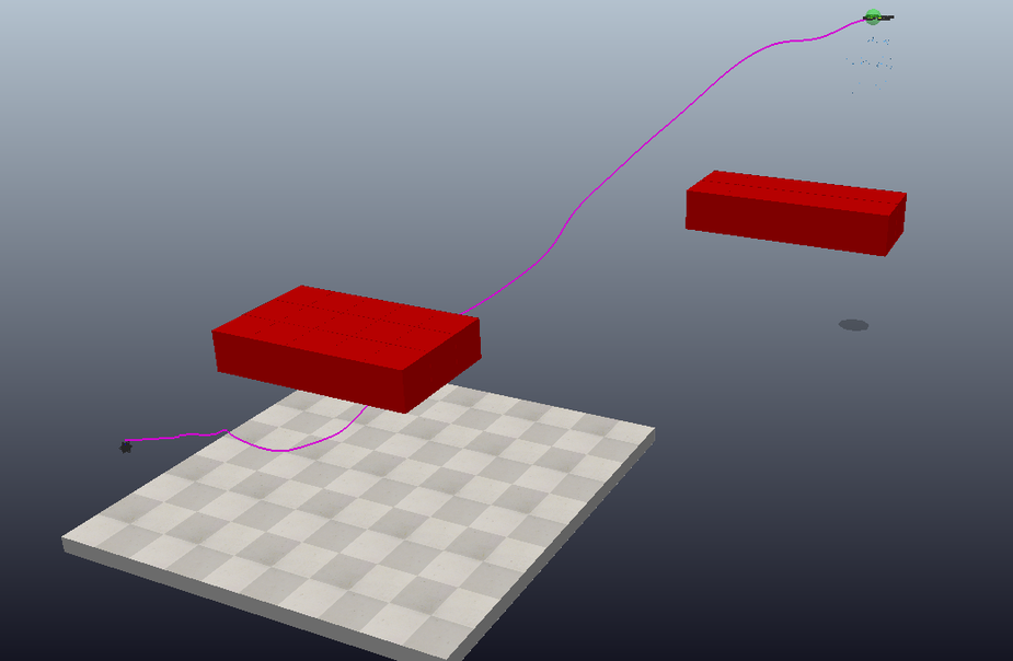
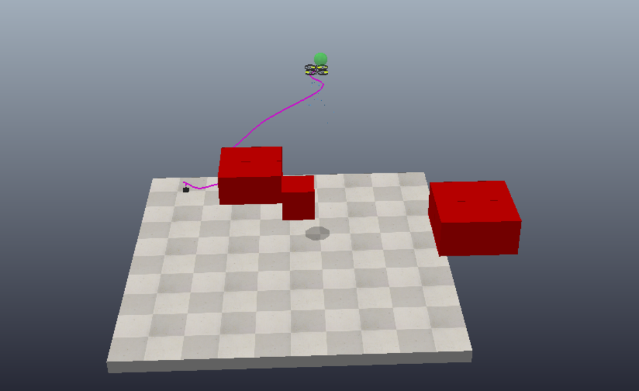
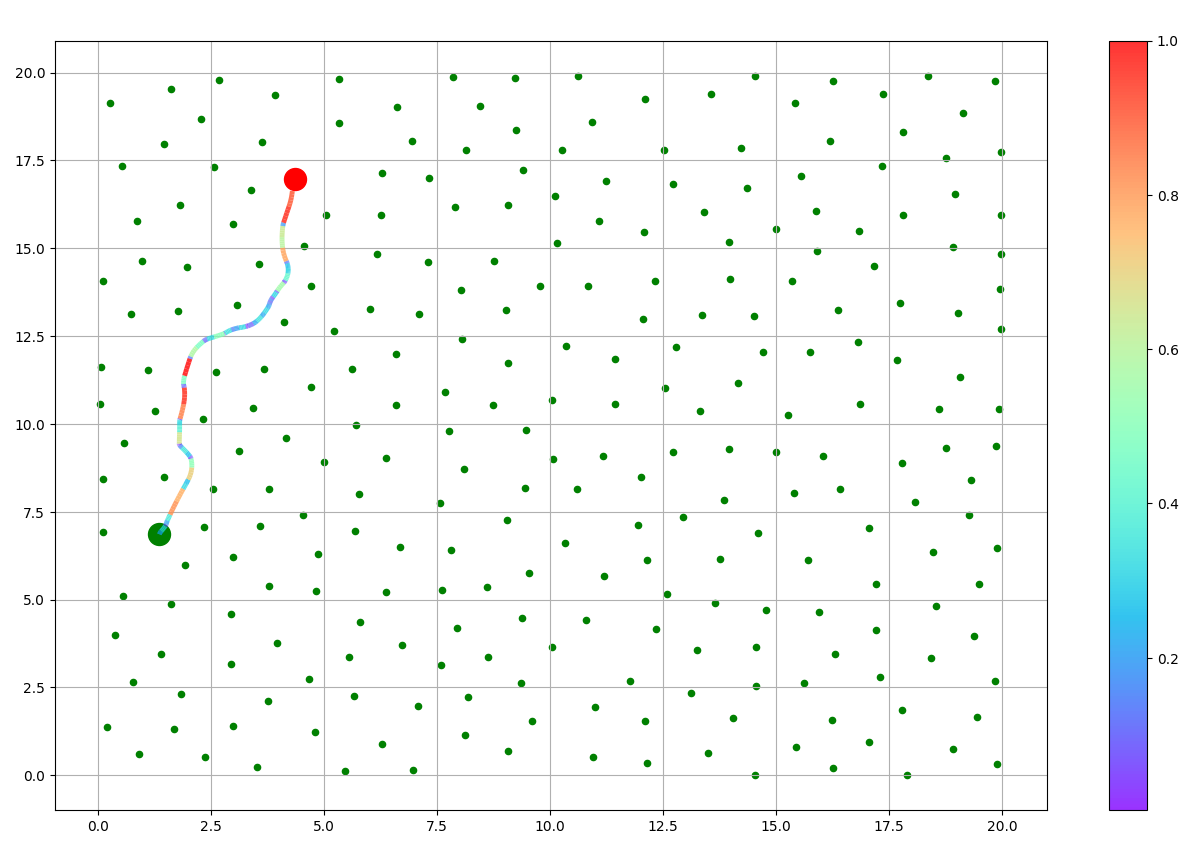
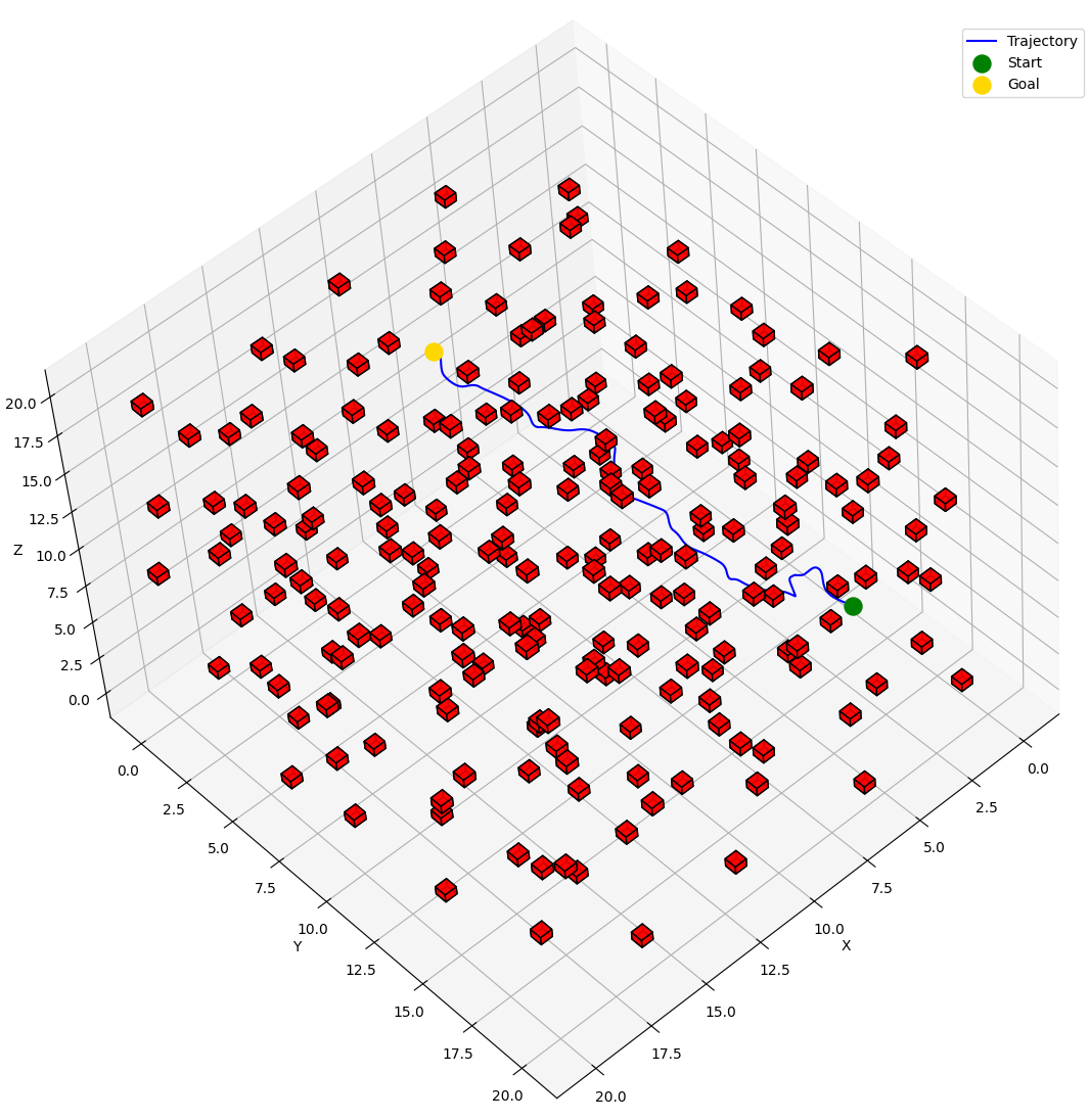
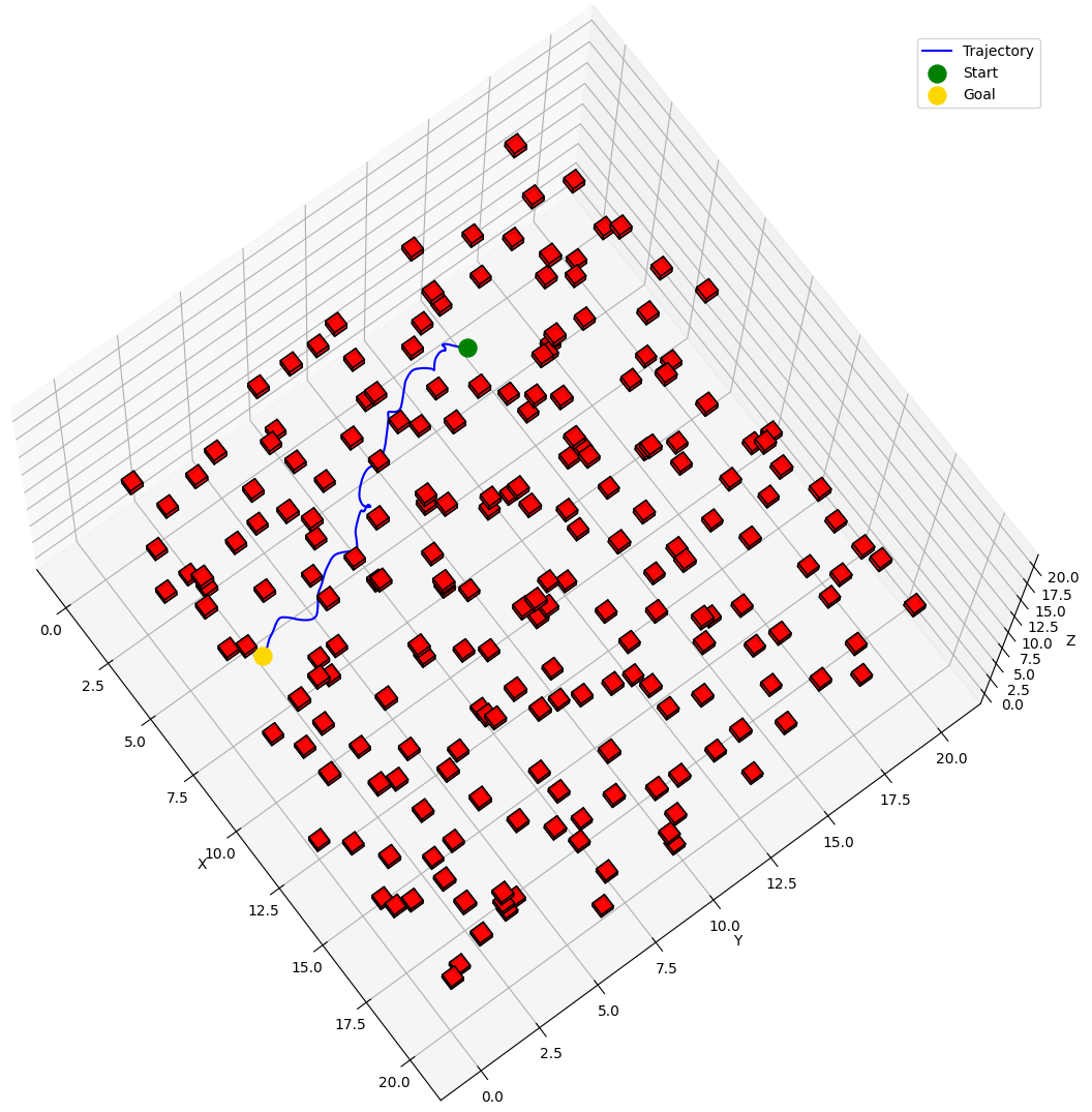
The BOW Planner is a motion planning algorithm that leverages constrained Bayesian optimization to expertly navigate robots through complex environments. By adeptly managing kinodynamic constraints such as velocity and acceleration limits, it ensures fast, secure, and near-optimal trajectory generation with remarkably few samples. Proven across real-world robotic systems, BOW stands out for its sample efficiency, safety-aware optimization, and scalability—making it a game-changer for robotic navigation.

BOW Environment CBO Samples
BOW efficiently finds optimal controls (white dots) with fewer samples (black dots) compared to traditional methods.

Key Contributions

The BOW Planner introduces several novel advancements in motion planning:

  • Constrained Bayesian Optimization: Integrates safety and kinodynamic constraints directly into the optimization process, ensuring feasible and efficient trajectories.
  • Window-Based Approach: Optimizes over sliding windows of control sequences, balancing computational speed with long-term planning accuracy.
  • Sample Efficiency: Achieves high-quality trajectories with significantly fewer samples than traditional methods like MPPI or RRT, as demonstrated in benchmark results.
  • Scalability: Proven effective across diverse robotic systems (UGVs and UAVs) in complex, high-dimensional environments with real-time performance.

Unmanned Ground Vehicle Experiments

We implemented the BOW Planner for a non-holonomic differential wheel robot navigating through a 2D space with obstacles. Experiments were conducted across five simulated environments and replicated in CoppeliaSim. The robot’s state is a 5D vector (position, orientation, linear and angular velocities), with control inputs as linear and angular velocities. BOW demonstrated rapid navigation and obstacle avoidance, even treating other robots as dynamic obstacles in multi-robot scenarios.

Environment 1 Environment 2 Environment 3 Environment 4
Environment 5 Environment 6 Environment 7
Seven simulated 20m×20m environments where black squares represent obstacles in the first five environments, and the sixth environment features non-convex obstacles composed of clustered green triangles. The seventh shows bug trap results. The curved trajectories display a blue-to-red gradient indicating increasing linear velocity from low to high.
BOW Planner performance in a simulated UGV environment with static obstacles.
Real-world UGV navigation with static and dynamic obstacle avoidance using BOW.
Performance evaluation of the BOW Planner in a real-world UGV environment with static obstacles, utilizing an onboard Lidar sensor. The generated occupancy map accurately represents the environmental layout while the robot demonstrates successful trajectory tracking using BOW.

Unmanned Aerial Vehicle Experiments

To demonstrate scalability, the BOW Planner was applied to a 6DOF aerial robot in a 3D environment with obstacles. The robot’s state is a 12D vector (position, velocity, orientation, and their derivatives), with control inputs as linear velocities and yaw rate. Evaluated in both CoppeliaSim simulations and real-world tests, BOW efficiently navigated UAVs through varied obstacle densities (0.04–0.14) and dispersities (2.38–4.15), achieving planning times as low as 5.64 ms.

UAV Env 1 UAV Env 2 UAV Env 3 UAV Env 4 UAV Env 5
Five simulated 3D environments for UAVs using BOW in CoppeliaSim (red cubes are obstacles).
BOW Planner performance in a simulated UAV 3D environment with static obstacles in CoppeliaSim.
Real-world UAV navigation through 3D environments with obstacles using BOW.

Experiments in Poisson Forest Environment for Both UAV and UGV

We implemented the BOW Planner for a non-holonomic differential wheel robot and a UAV navigating through 2D and 3D Poisson forest environments, respectively. Experiments were conducted in procedurally generated forest environments with obstacles distributed using Poisson sampling to mimic natural, non-uniform obstacle patterns. BOW demonstrated robust navigation and obstacle avoidance in complex organic obstacle arrangements, validated through three trials each for UGV and UAV platforms.

UGV Trial 1 UGV Trial 2 UGV Trial 3
BOW planner performance for UGV in three 2D Poisson forest environments with obstacle densities of 1.0, 1.5, and 2.0 per m². The green and red dots denote the start and goal positions, respectively, with curved trajectories showing a blue-to-red gradient indicating increasing linear velocity.
UAV Trial 1 UAV Trial 2 UAV Trial 3
BOW planner performance for UAV in three 3D Poisson forest environments with obstacle density of 1.0, 2.0, and 3.0 per m³. The green and gold spheres denote the start and goal positions, respectively, with trajectories shown with a blue line.

Benchmark Results

The BOW Planner was benchmarked against RRT, DWA, MPPI, HRVO, and CBF across five environments with varying obstacle densities (5.02%–8.30%) and dispersities (2.59%–6.20%). BOW consistently achieved the fastest planning times (28.2–78.6 ms) and per-step execution (0.17–0.26 ms), with competitive trajectory lengths (6.88–19.49 m), outperforming others in computational efficiency. The table below summarizes performance across all five environments.

Env Method Lib. + Lang Steps Traj. Length (m) Total Time (ms) Time/Step (ms) Avg Velocity Avg Jerk
1 BOW FCL + C++ 161.2 ± 2.9 14.14 ± 0.09 23.26 ± 0.35 0.14 0.947 ± 0.020 0.190 ± 0.024
DWA FCL + C++ 157.0 ± 0.00 14.33 ± 0.00 103.68 ± 2.07 0.66 0.952 ± 0.00 0.031 ± 0.000
HRVO C++ 539.0 ± 0.00 15.78 ± 0.00 269.22 ± 7.21 0.50 0.293 ± 0.00 0.223 ± 0.00
RRT FCL + C++ 55.2 ± 8.0 17.39 ± 1.38 389.83 ± 272.41 7.06 0.796 ± 0.038 0.849 ± 0.062
MPPI CUDA + Py 137.0 ± 0.00 13.98 ± 0.00 5865.90 ± 182.73 42.82 1.654 ± 0.052 -1.150 ± 0.108
CBF Gurobi + Py 156.0 ± 0.00 14.42 ± 0.00 9892.10 ± 97.26 63.41 0.992 ± 0.010 -0.020 ± 0.001
2 BOW FCL + C++ 160.5 ± 3.2 14.21 ± 0.08 23.09 ± 0.59 0.14 0.955 ± 0.022 0.188 ± 0.026
DWA FCL + C++ 332.0 ± 0.00 30.26 ± 0.00 83.15 ± 1.78 0.25 1.032 ± 0.000 0.040 ± 0.000
HRVO C++ 341.0 ± 0.00 14.87 ± 0.00 282.89 ± 7.65 0.83 0.436 ± 0.00 0.137 ± 0.00
RRT FCL + C++ 57.0 ± 10.2 17.30 ± 2.56 464.82 ± 87.55 8.15 0.765 ± 0.036 0.859 ± 0.085
MPPI CUDA + Py 156.0 ± 0.00 14.38 ± 0.00 6625.00 ± 146.45 42.47 1.467 ± 0.032 -2.647 ± 0.172
3 BOW FCL + C++ 199.2 ± 3.8 17.48 ± 0.06 28.14 ± 0.58 0.14 0.939 ± 0.020 0.190 ± 0.016
DWA FCL + C++ 220.0 ± 0.00 19.14 ± 0.00 102.50 ± 1.83 0.47 0.889 ± 0.000 0.028 ± 0.00
HRVO C++ 422.0 ± 0.00 20.07 ± 0.00 468.44 ± 10.51 1.11 0.476 ± 0.00 0.302 ± 0.000
RRT FCL + C++ 69.2 ± 12.7 20.69 ± 2.63 808.09 ± 533.78 11.68 0.783 ± 0.022 0.886 ± 0.050
MPPI CUDA + Py 150.0 ± 0.00 17.27 ± 0.00 6496.80 ± 346.90 43.31 1.774 ± 0.089 2.062 ± 0.291
CBF Gurobi + Py 151.0 ± 0.00 17.44 ± 0.00 12146.60 ± 185.49 80.44 0.930 ± 0.014 -0.018 ± 0.001
4 BOW FCL + C++ 210.8 ± 6.5 18.67 ± 0.12 30.90 ± 0.68 0.15 0.945 ± 0.036 0.172 ± 0.028
DWA FCL + C++ 373.0 ± 0.00 34.33 ± 0.00 169.20 ± 3.58 0.45 0.970 ± 0.00 0.030 ± 0.00
HRVO C++ 465.0 ± 0.00 21.06 ± 0.00 676.32 ± 12.82 1.45 0.453 ± 0.00 0.341 ± 0.000
RRT FCL + C++ 77.9 ± 10.0 23.68 ± 2.67 745.79 ± 406.64 9.57 0.769 ± 0.021 0.898 ± 0.072
MPPI CUDA + Py 198.0 ± 0.00 18.86 ± 0.00 8674.80 ± 156.41 43.81 vyp 1.467 ± 0.026 0.194 ± 0.010
CBF Gurobi + Py 171.0 ± 0.00 18.09 ± 0.00 15135.40 ± 335.45 88.51 0.805 ± 0.018 -0.002 ± 0.000
5 BOW FCL + C++ 95.0 ± 5.4 7.56 ± 0.19 12.89 ± 0.09 0.14 1.007 ± 0.077 0.357 ± 0.052
HRVO C++ 204.0 ± 0.00 8.34 ± 0.00 369.20 ± 2.49 1.81 0.409 ± 0.000 0.260 ± 0.00
RRT FCL + C++ 31.7 ± 3.7 9.53 ± 0.80 93.18 ± 56.97 2.94 0.785 ± 0.035 0.927 ± 0.100
MPPI CUDA + Py 139.0 ± 0.00 8.86 ± 0.00 5983.00 ± 183.18 43.04 0.691 ± 0.021 -0.930 ± 0.086
6 BOW FCL + C++ 101.9 ± 5.1 8.73 ± 0.09 10.00 ± 0.33 0.10 0.940 ± 0.063 0.158 ± 0.029
DWA FCL + C++ 556.0 ± 0.00 25.36 ± 0.00 589.78 ± 4.04 1.06 0.556 ± 0.00 0.043 ± 0.00
RRT FCL + C++ 36.1 ± 8.1 10.54 ± 1.56 128.16 ± 79.40 3.55 0.757 ± 0.041 0.811 ± 0.060
MPPI CUDA + Py 1048.0 ± 0.00 29.94 ± 0.00 44312.20 ± 645.95 42.28 0.056 ± 0.001 0.421 ± 0.018
Comparison of path planning methods across six environments. Best values for each environment are highlighted in bold.

Authors

Anonymous Authors


Citation

@article{anonymous2025bow,
    author = {Anonymous},
    title = {BOW: Bayesian Optimization over Windows for Motion Planning in Complex Environments},
    journal = {},
    year = {2025},
}